GraphSX

GraphSX is a JSX-like DSL for drawing diagrams, plots, and Markdown-native figures as SVG.

Playground · VS Code Extension

It is designed for notes, papers, docs, and small scientific figures where the source should stay readable:

• JSX-like tags and props instead of a separate command language
• reusable shapes with public ports
• links, explicit paths, routing, arrowheads, and labels
• standalone plots with axes, data, ticks, legends, annotations, and KaTeX labels
• nested plots inside graphs for subplots and mixed plot/diagram figures
• Markdown fences and CodeMirror live-preview widgets
• a small TikZ-subset importer for common node, draw, coordinate, and pic diagrams

Try the playground: https://slxuphys.github.io/graphsx/

Install the VS Code extension: https://marketplace.visualstudio.com/items?itemName=slxuphys.graphsx-vscode

Current npm package name: @slxu/graphsx. Project and repo name: GraphSX.

Install from npm:

npm install @slxu/graphsx

Optional integrations use the host app's packages:

npm install katex markdown-it
npm install codemirror @codemirror/state @codemirror/view @codemirror/lang-javascript @codemirror/lang-markdown

What It Looks Like

Port Diagram

<Graph>
  <Style id="box" fill="#eef6ff" stroke="#1d4ed8" />
  <Style id="wire" stroke="#7c3aed" strokeWidth={3} />

  <Rect id="A" at={[70, 82]} size={[100, 60]} label="alpha" useStyle="box">
    <Port id="out" right label="xy" />
  </Rect>
  <Circle id="B" at={[280, 112]} r={40} label="B">
    <Port id="in" left />
  </Circle>

  <Link headArrow from="A.out" to="B.in" useStyle="wire" />
</Graph>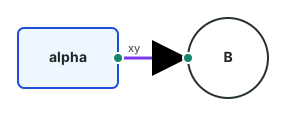

Parametric Plot

<Plot width={430} height={330} xDomain={[-18, 18]} yDomain={[-18, 14]} frame box>
  <Data
    id="heart"
    x="16 * pow(sin(t), 3)"
    y="13*cos(t) - 5*cos(2*t) - 2*cos(3*t) - cos(4*t)"
    domain={[0, 2*pi]}
    samples={360}
  />

  <Axis x label="x" ticks grid />
  <Axis y label="y" ticks grid />
  <Line data="heart" stroke="#e11d48" strokeWidth={2.6} />
</Plot>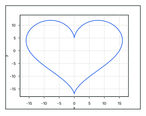

Reusable Shapes And Repeat

<Graph route="straight">
  <Shape id="Tensor" groupBox={false}>
    <Rect id="box" size={[54, 54]} corner={8} label={tensorLabel}>
      <Port id="left" left r={0} />
      <Port id="right" right r={0} />
      <Port id="phys" bottom r={0} />
    </Rect>
    <Port id="left" target="box.left" />
    <Port id="right" target="box.right" />
    <Port id="phys" target="box.phys" />
  </Shape>

  <Repeat count={4} as="i" step={[96, 0]}>
    <Tensor id={`A${i}`} at={[70, 60]} tensorLabel={`A${i}`} />
  </Repeat>
</Graph>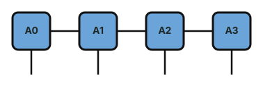

Quick Example

<Graph>
  <Style id="box" fill="#eef6ff" stroke="#1d4ed8" strokeWidth={2} />
  <Style id="wire" stroke="#7c3aed" strokeWidth={3} />

  <Rect id="A" at={[100, 100]} size={[100, 60]} label="$\alpha$" useStyle="box">
    <Port id="out" right label="xy" />
  </Rect>

  <Circle id="B" at={[300, 100]} r={40} label="B">
    <Port id="in" left />
  </Circle>

  <Link headArrow from="A.out" to="B.in" useStyle="wire" />
</Graph>

Use it from JavaScript:

import { parseGraphSXDocument, renderGraphSXDocument } from "@slxu/graphsx";
import katex from "katex";

const model = parseGraphSXDocument(source);
renderGraphSXDocument(document.querySelector("svg"), model, { katex });

Display-list builders can also ask the host for exact text/math sizes. If these hooks are omitted, GraphSX uses built-in estimates:

import { buildGraphDisplayList, parseGraph } from "@slxu/graphsx";

const graph = parseGraph(source);
const display = buildGraphDisplayList(graph, {
  measure: {
    math: (source, style) => measureKaTeX(source, style),
    text: (text, style) => measureCanvasText(text, style)
  }
});

Labels are opt-in. Use label="xy" for plain text and label="$\alpha$" for KaTeX math. If there is no label prop, no label is rendered.

TikZ-subset input is parsed separately from GraphSX:

import { parseTikz, renderTikz } from "@slxu/graphsx/tikz";

const model = parseTikz(tikzSource, { units: { cm: 80, pt: 1.3333333333 } });
renderTikz(document.querySelector("svg"), model, { katex });

Syntax Model

GraphSX should feel familiar if you already understand JSX:

• tags define components: <Rect />, <Plot />, <Shape />
• props configure components: at={[100, 80]}, label="$x$", frame
• children nest inside parents: ports inside shapes, ticks inside axes
• braces hold static values and simple arithmetic: {[L / 2, 20]}
• backtick strings support substitution: label={`$A^{[${site}]}$`}

GraphSX is not a full JSX compiler. Values are parsed by a small safe parser, not by executing arbitrary JavaScript.

Styling

Most visible components can be styled inline:

<Rect id="A" style={{ fill: "#eef6ff", stroke: "#1d4ed8", strokeWidth: 2 }} />
<Link from="A.right" to="B.left" style={{ stroke: "#7c3aed", strokeWidth: 3 }} />

Or with reusable style libraries:

<Graph>
  <Style id="tensor" fill="#6aa4d8" stroke="#111111" strokeWidth={3} />
  <Style id="wire" stroke="#111111" strokeWidth={2.5} />

  <Rect id="A" useStyle="tensor" />
  <Link from="A.right" to="B.left" useStyle="wire" />
</Graph>

Inline style overrides useStyle. Style keys can use camelCase, such as strokeWidth; the renderer maps them to SVG attributes.

Plot-specific boxes also support dedicated style props, such as frameStyle, boxStyle, textStyle, and labelStyle.

Graphs

<Graph> is the general figure canvas. It auto-sizes around its content and supports nodes, ports, links, paths, reusable shapes, repeats, and nested plots.

Canonical built-in graph nodes:

• Rect
• Circle
• Point, Anchor
• Plot when placed inside a graph

Rect, Circle, and nested Plot expose default ports:

A.left
A.right
A.top
A.bottom

Point and Anchor expose:

J.center

Ports

Ports can use side shorthand or custom local coordinates:

<Rect id="A" at={[100, 100]} size={[120, 80]}>
  <Port id="in" left />
  <Port id="tap" at={[60, 20]} angle={35} label="$t$" />
</Rect>

at on a port is relative to its shape. angle controls the direction a routed link emits from or enters the port. 0 points right, 90 points down, 180 points left, and -90 points up.

Links

Links connect quoted port addresses:

<Link headArrow from="A.right" to="B.left" />

Routing options:

<Graph route="auto" grid={20} padding={16} corner={8}>
  <Rect id="A" at={[60, 100]} size={[90, 60]} />
  <Rect id="Block" at={[210, 70]} size={[90, 110]} />
  <Rect id="B" at={[380, 100]} size={[90, 60]} />

  <Link headArrow from="A.right" to="B.left" />
  <Link headArrow from="A.top" to="B.top" route="orthogonal" corner={0} />
</Graph>

Available routes:

• default curved route
• route="straight"; add signed offset for a connected parallel detour
• route="orthogonal"
• route="bypass" with side and offset for residual/skip-style detours
• route="auto" for first-pass obstacle avoidance

route="auto" avoids shape boxes. It does not yet optimize for edge crossings.

Bypass routes make rounded orthogonal detours around a chosen side:

<Link from="A.right" to="B.left" route="straight" offset={12} />
<Link from="A.top" to="B.left" route="bypass" side="left" offset={48} corner={16} headArrow />

Paths

Use <Path> for exact geometry rather than semantic port-to-port links:

<Graph>
  <Path points={[[90, 80], [90, 240], [180, 240]]} />
  <Path points={[[120, 80], [170, 80], [170, 160]]} corner={6} headArrow />
  <Path d="M 90 80 L 180 80" tailArrow arrowSize={8} />
</Graph>

Path accepts points or raw SVG d. Add headArrow, tailArrow, and arrowSize for arrows. corner rounds bends in point paths.

Layout

Coordinates are optional when graph layout is enabled:

<Graph layout="dag" direction="right" rankGap={200} nodeGap={90}>
  <Rect id="A" size={[100, 60]} />
  <Rect id="B" size={[100, 60]} />
  <Rect id="C" size={[100, 60]} />

  <Link headArrow from="A.right" to="B.left" />
  <Link headArrow from="A.right" to="C.left" />
</Graph>

Supported layouts:

• layout="row"
• layout="column"
• layout="dag"

Explicit at={[x, y]} positions win over automatic layout.

Reusable Shapes

Define custom shapes with <Shape>, then instantiate them by tag name:

<Graph>
  <Shape id="Tensor" groupBox={false}>
    <Rect id="box" at={[0, 0]} size={[56, 56]} corner={8} label={`$A^{[${site}]}$`} />
    <Port id="left" target="box.left" />
    <Port id="right" target="box.right" />
    <Port id="phys" target="box.bottom" />
  </Shape>

  <Repeat count={4} as="i" step={[100, 0]}>
    <Tensor id={`A${i}`} at={[100, 100]} site={i} />
  </Repeat>

  <Repeat count={3} as="i">
    <Link from={`A${i}.right`} to={`A${i+1}.left`} />
  </Repeat>
</Graph>

Address paths use ids. A0.left is the public port on the Tensor instance. A0.box.left is the left port on the internal child rectangle.

Grouped shapes render a dashed group box by default. Use groupBox={false} on the shape definition or on an instance to hide it.

Shape variants can inherit from another shape:

<Shape id="Gate" groupBox={false}>
  <Rect id="box" size={[70, 40]} label={label} />
  <Port id="in" target="box.left" />
  <Port id="out" target="box.right" />
</Shape>

<Shape id="WideGate" from="Gate" w={110} label="$U$" />

Derived shapes can override props, but not replace inherited children with the same id.

Repeat

Use <Repeat> to expand repeated nodes, links, paths, or shape internals:

<Graph>
  <Repeat count={2} as="row" step={[0, 90]}>
    <Repeat count={3} as="col" step={[100, 0]}>
      <Rect id={`cell-${row}-${col}`} at={[100, 100]} size={[70, 50]} label={`cell ${row},${col}`} />
    </Repeat>
  </Repeat>
</Graph>

step offsets each repeated copy. Backtick strings can use ${i}, ${i+1}, ${row}, ${col}, and simple arithmetic.

Plots

<Plot> can be used standalone:

<Plot width={560} height={340} xDomain={[0, 2*pi]} yDomain={[-1.2, 1.2]} frame box>
  <Data id="sin" y="sin(x)" domain={[0, 2*pi]} samples={160} />

  <Axis x label="$x$">
    <Ticks
      values={[0, pi/2, pi, 3*pi/2, 2*pi]}
      labels={["$0$", "$\pi/2$", "$\pi$", "$3\pi/2$", "$2\pi$"]}
      grid
    />
  </Axis>
  <Axis y label="$\sin(x)$" ticks grid />

  <Line data="sin" stroke="#2563eb" strokeWidth={2} label="$\sin(x)$" />
  <Legend />
</Plot>

Or inside a graph as a placed subplot:

<Graph>
  <Plot id="left" at={[0, 0]} width={320} height={220} frame box>
    <Port id="out" right />
    <Axis x ticks />
    <Axis y ticks />
    <Line points={[[0, 1], [1, 2], [2, 4]]} />
  </Plot>

  <Plot id="right" at={left.right + [90, 0]} width={320} height={220} frame box>
    <Port id="in" left />
    <Axis x ticks />
    <Axis y ticks />
    <Line points={[[0, 4], [1, 2], [2, 1]]} />
  </Plot>

  <Link from="left.out" to="right.in" headArrow />
</Graph>

In a plot:

• frame draws the outer plot panel
• box draws the inner axis/data box
• padding controls the gap between frame and axes
• xDomain and yDomain set data coordinates
• Data can hold points, x/y arrays, or generated math data
• generated Data always stores point fields named x and y
• parametric data uses x="..." and y="..."; the default sampling variable is t
• Line, Curve, Mark, Scatter, Text, Legend, and annotation shapes render on top
• generated data expressions may be complex; plotted coordinates use the real part by default

Parametric curves sample a variable and evaluate both coordinates:

<Plot width={500} height={460} xDomain={[-18, 18]} yDomain={[-18, 14]} frame box>
  <Data
    id="heart"
    x="16 * pow(sin(t), 3)"
    y="13*cos(t) - 5*cos(2*t) - 2*cos(3*t) - cos(4*t)"
    domain={[0, 2*pi]}
    samples={420}
  />
  <Line data="heart" stroke="#e11d48" strokeWidth={2.8} />
</Plot>

For y="..." alone, the default sampling variable is x, and the sampled domain value is stored as the point's x field. For x="..." plus y="...", the default sampling variable is t; both expressions are evaluated from that variable and stored as point fields named x and y. Use variable="theta" to override either default.

<Data id="phase" y="exp(1j*t)" variable="t" domain={[0, 2*pi]} />

This stores points like { x: t, y: exp(1j*t) }.

Complex math uses Python-style imaginary literals such as 1j, 2.5j, and x + 3j. Bare j is just a normal variable name, so exp(j*x) only works if j is declared in params.

<Plot width={560} height={340} xDomain={[-1, 1]} yDomain={[-1.1, 1.1]} frame box>
  <Data id="root" y="sqrt(x)" domain={[-1, 1]} samples={200} />

  <Axis x label="$x$" ticks grid />
  <Axis y label="$\sqrt{x}$" ticks grid />

  <Line data="root" label="real" />
  <Line data="root" yMap="imag(y)" stroke="#dc2626" label="imag" />
  <Line data="root" yMap="abs(y)" stroke="#16a34a" label="abs" />
  <Legend />
</Plot>

Use xMap and yMap to transform stored points at plot time. The map scope contains the stored x and y values, which may be real or complex. Either map can use either stored field:

<Plot width={420} height={420} xDomain={[-1.2, 1.2]} yDomain={[-1.2, 1.2]} frame box>
  <Data id="phase" y="exp(1j*t)" variable="t" domain={[0, 2*pi]} samples={240} />

  <Line data="phase" xMap="real(y)" yMap="imag(y)" label="unit circle" />
</Plot>

Plot annotations can use Rect, Circle, Anchor, Link, and Path:

<Plot width={500} height={300} xDomain={[0, 5]} yDomain={[0, 10]} frame box>
  <Line points={[[0, 1], [2, 4], [5, 9]]} />
  <Circle id="peak" at={[5, 9]} r={5} fill="#ef4444" />
  <Rect id="note" at={[3.2, 8.2]} size={[90, 28]} label="peak">
    <Port id="tip" left />
  </Rect>
  <Link from="note.tip" to="peak.top" headArrow />
</Plot>

Annotation coordinates default to data coordinates. Use atUnit="screen" for screen/SVG coordinates.

Supported Tags

Common top-level tags:

| Tag | Children | Key props | | --- | --- | --- | | Graph | Style, Shape, nodes, Plot, Link, Path, Repeat | route, layout, direction, grid, padding, corner | | Plot | plot children, and Port when nested in Graph | width, height, padding, xDomain, yDomain, frame, box |

Graph tags:

| Tag | Children | Key props | | --- | --- | --- | | Rect | Port | id, at, size, w, h, label, corner, anchor, origin, rotate, flipX, flipY, style, useStyle | | Circle | Port | id, at, r, label, anchor, origin, rotate, flipX, flipY, style, useStyle | | Point, Anchor | Port | id, at, label, r, style, useStyle | | Port, Leg | none | id, left, right, top, bottom, side, at, angle, target, label, r, style, useStyle | | Link | none | from, to, route, side, offset, corner, stub, headArrow, tailArrow, arrowSize, style, useStyle | | Path | none | points, d, at, corner, closed, headArrow, tailArrow, arrowSize, rotate, flipX, flipY, style, useStyle | | Shape | graph nodes, Port, Link, Path, Repeat | id, from, groupBox, user-defined props | | Repeat | repeatable graph children | count, as, step | | Style | none | id, SVG style props |

Plot tags:

| Tag | Children | Key props | | --- | --- | --- | | Data | none | id, points, x, y, domain, samples, params, variable | | Axis | Ticks | x, y, label, ticks, grid, labelGap, tickLabelGap, tickSize, style, labelStyle | | Ticks | none | values, labels, grid, labelGap, tickLabelGap, tickSize, style, labelStyle | | Line, Curve | none | data, points, x, y, xMap, yMap, fmt, label, animate, stroke, strokeWidth, fill, r, style, useStyle | | Mark, Scatter | none | data, at, points, x, y, xMap, yMap, r, label, animate, fill, stroke, style, useStyle | | Text, Label | none | at, label, fontSize, anchor, baseline, rotate, style, useStyle | | Legend | none | position, box, padding, margin, fontSize, textStyle, boxStyle |

Canonical tags use PascalCase. A few aliases are accepted for convenience, but new examples should prefer the canonical form:

| Canonical | Aliases | | --- | --- | | Rect | rect, Rec, rec | | Circle | circle, Circ, circ | | Point | point | | Anchor | anchor | | Path | path | | Data | Dataset | | Axis | XAxis, YAxis | | Ticks | ticks | | Curve | Series | | Legend | legend |

TikZ Subset

GraphSX also includes a separate TikZ-subset importer. It is intentionally orthogonal to the JSX-like GraphSX parser: TikZ source is parsed by the TikZ importer, then rendered through the same display-list/SVG layer.

\tikzset{
  gateStyle/.style={rectangle, draw=black, fill=white!5, very thick, minimum width=1.1cm, minimum height=.55cm},
  one gate/.pic={
    \node[gateStyle] (-body) at (0,0) {$U$};
    \coordinate (-left) at (-body.west);
    \coordinate (-right) at (-body.east);
  }
}

\begin{tikzpicture}
  \pic (u1) at (0,0) {one gate};
  \pic (u2) at (2,0) {one gate};
  \draw[->, thick] (u1-right) -- (u2-left);
\end{tikzpicture}

Supported v1 commands include:

• \node[...] (id) at (...) {...};
• \coordinate (id) at (...);
• \draw[...] (...) -- (...), |-, and -|
• \filldraw[...] (...) circle (...);
• \tikzset{name/.style={...}}
• \tikzset{name/.pic={...}} with \pic (id) at (...) {name};

Reusable pic definitions support local names that begin with -. For example (-left) inside a pic becomes u1-left when instantiated as \pic (u1) ....

The importer supports common styles such as rectangle, circle, draw, fill, thick, very thick, dashed, ->, <-, <->, minimum width, minimum height, minimum size, and rounded corners. It is not a full TeX/TikZ engine, so arbitrary TeX macros and advanced TikZ libraries are outside the v1 scope.

Markdown

GraphSX works in Markdown with a markdown-it plugin:

import MarkdownIt from "markdown-it";
import katex from "katex";
import { graphsxMarkdownIt, renderGraphSXBlocks } from "@slxu/graphsx";
import "@slxu/graphsx/markdown.css";

const md = new MarkdownIt().use(graphsxMarkdownIt);
const preview = document.querySelector("#preview");

preview.innerHTML = md.render(markdownSource);
renderGraphSXBlocks(preview, { katex });

Authors use graphsx fences:

```graphsx
<Graph>
  <Rect id="A" />
  <Rect id="B" at={[220, 0]} />
  <Link headArrow from="A.right" to="B.left" />
</Graph>
```

Reusable style/shape libraries can be declared with hidden graphsx-defs fences:

```graphsx-defs theme
<Style id="tensor" fill="#6aa4d8" stroke="#111111" />
<Style id="wire" stroke="#111111" strokeWidth={2.5} />
```

```graphsx use="theme"
<Graph>
  <Rect id="A" useStyle="tensor" />
  <Rect id="B" at={[120, 0]} useStyle="tensor" />
  <Link from="A.right" to="B.left" useStyle="wire" />
</Graph>
```

Multiple library names can be separated by spaces or commas.

TikZ-subset diagrams use a separate fence:

```graphsx-tikz
\begin{tikzpicture}
  \node[rectangle, draw=black] (A) at (0,0) {A};
\end{tikzpicture}
```

CodeMirror Live Preview

Use the CodeMirror extension to render graphsx fences as editable live widgets inside a Markdown editor:

import { EditorView, basicSetup } from "codemirror";
import { markdown } from "@codemirror/lang-markdown";
import { jsxLanguage } from "@codemirror/lang-javascript";
import { graphsxCodeMirrorLivePreview } from "@slxu/graphsx/codemirror";
import "@slxu/graphsx/codemirror.css";

new EditorView({
  doc,
  extensions: [
    basicSetup,
    markdown({
      codeLanguages: (info) => {
        const name = info.trim().split(/\s+/)[0];
        return name === "graphsx" || name === "graphsx-defs" || name === "graphsx-tikz" ? jsxLanguage : null;
      }
    }),
    graphsxCodeMirrorLivePreview({ katex })
  ],
  parent: document.querySelector("#editor")
});

When the cursor is outside a graphsx fence, the fence renders as an SVG widget. Clicking the widget moves the cursor into the original fenced code. graphsx-defs fences render as compact library markers and feed reusable shapes/styles to later fences.

VS Code Extension

This repo also contains a VS Code extension in packages/vscode-graphsx. It teaches VS Code's built-in Markdown preview and Jupyter notebook Markdown cells to render graphsx fenced blocks.

Install it from the Visual Studio Marketplace: https://marketplace.visualstudio.com/items?itemName=slxuphys.graphsx-vscode

Build the extension bundle from the repo root:

npm run build:vscode

Development

npm install
npm test
npm run playground

The playground runs at the Vite URL printed in your terminal, usually http://127.0.0.1:5173/.

Build the GitHub Pages version:

npm run build:pages

Notes

• Graph labels and plot labels support KaTeX when a katex instance is passed to the renderer.
• Graph <Plot> nodes behave like rectangles: they have at, width, height, and default side ports.
• Standalone <Plot> is best for one plot. Use <Graph> when you want subplots or a mixed figure.
• The parser intentionally supports a constrained JSX-like subset rather than arbitrary JavaScript.